Tuto@MATE

Les modèles en équations structurelles

Solenne Roux

(LabPsy - UR4139 - Université de Bordeaux)

Ce que ne sont pas les SEM

Ce que sont les SEM

Photo de Henry Be sur Unsplash

Photo de Tom Hermans sur Unsplash

Les SEM en SHS

Lost in Translation

Modèles en équations structurales (MES) / Structural Equations Modeling (SEM)

Modèles structuraux

Modèles en équations structurales (MES) / Structural Equations Modeling (SEM)

Modèles structuraux

Modèles en équations simultanées

Modèles en pistes causales / Path analysis

Analyses factorielles confirmatoires (AFC) / Confirmatory factorial analysis (CFA)

Médiation / Modération

Latent Class Analysis (LCA) / Latent Profile Analysis (LPA)

…

Perspective historique des SEM

1920 - Wright, S., - Biologie - Path Analysis

1928 - Wright, P., - Economie - Path Analysis + Modèles à équations simultanées

Années 50 - Sociologie - Modèles causaux

1970 - Jöreskog - Psychologie - LSEM

1980 - Bentler - Psychologie - Modélisation plus complexe (effets indirects, etc.)

Depuis début 2000 - Explosion des SEM et diversification des modèles

Lost in Translation II

Les SEM - Méthode de factorisation ?

Exemple : Black Cat Biais

Black Cat Biais : Prevalence and Predictors

Les modèles théoriques s’ajustent-ils à nos données ?

Mesure du rapport à la religion

attach(datSCSRFQp) # Attacher car lavaan refuse les $

modelS <- 'F_SCSRF  =~ SCSRF1 + SCSRF2 + SCSRF3 + SCSRF4 + SCSRF5 + SCSRF6 + SCSRF7 + SCSRF8 + SCSRF9 + SCSRF10'

fitMLRS <- cfa (modelS, std.lv=T, estimator="MLR", data=datSCSRFQp)
summary(fitMLRS, standardized=T, modindices = T, fit.measures=T)

lavaan 0.6.16 ended normally after 13 iterations

  Estimator                                         ML
  Optimization method                           NLMINB
  Number of model parameters                        20

  Number of observations                           749

Model Test User Model:
                                              Standard      Scaled
  Test Statistic                                41.369      42.416
  Degrees of freedom                                35          35
  P-value (Chi-square)                           0.212       0.182
  Scaling correction factor                                  0.975
    Yuan-Bentler correction (Mplus variant)                       

Model Test Baseline Model:

  Test statistic                              2551.350    2609.790
  Degrees of freedom                                45          45
  P-value                                        0.000       0.000
  Scaling correction factor                                  0.978

User Model versus Baseline Model:

  Comparative Fit Index (CFI)                    0.997       0.997
  Tucker-Lewis Index (TLI)                       0.997       0.996
                                                                  
  Robust Comparative Fit Index (CFI)                         0.997
  Robust Tucker-Lewis Index (TLI)                            0.996

Loglikelihood and Information Criteria:

  Loglikelihood user model (H0)              -9363.374   -9363.374
  Scaling correction factor                                  0.982
      for the MLR correction                                      
  Loglikelihood unrestricted model (H1)      -9342.690   -9342.690
  Scaling correction factor                                  0.978
      for the MLR correction                                      
                                                                  
  Akaike (AIC)                               18766.749   18766.749
  Bayesian (BIC)                             18859.123   18859.123
  Sample-size adjusted Bayesian (SABIC)      18795.616   18795.616

Root Mean Square Error of Approximation:

  RMSEA                                          0.016       0.017
  90 Percent confidence interval - lower         0.000       0.000
  90 Percent confidence interval - upper         0.032       0.033
  P-value H_0: RMSEA <= 0.050                    1.000       1.000
  P-value H_0: RMSEA >= 0.080                    0.000       0.000
                                                                  
  Robust RMSEA                                               0.017
  90 Percent confidence interval - lower                     0.000
  90 Percent confidence interval - upper                     0.032
  P-value H_0: Robust RMSEA <= 0.050                         1.000
  P-value H_0: Robust RMSEA >= 0.080                         0.000

Standardized Root Mean Square Residual:

  SRMR                                           0.018       0.018

Parameter Estimates:

  Standard errors                             Sandwich
  Information bread                           Observed
  Observed information based on                Hessian

Latent Variables:
                   Estimate  Std.Err  z-value  P(>|z|)   Std.lv  Std.all
  F_SCSRF =~                                                            
    SCSRF1            0.640    0.033   19.201    0.000    0.640    0.641
    SCSRF2            0.682    0.035   19.375    0.000    0.682    0.683
    SCSRF3            0.626    0.037   17.037    0.000    0.626    0.626
    SCSRF4            0.638    0.033   19.531    0.000    0.638    0.639
    SCSRF5            0.624    0.037   16.998    0.000    0.624    0.624
    SCSRF6            0.696    0.033   21.202    0.000    0.696    0.696
    SCSRF7            0.654    0.034   19.290    0.000    0.654    0.655
    SCSRF8            0.648    0.034   19.174    0.000    0.648    0.649
    SCSRF9            0.637    0.034   18.678    0.000    0.637    0.639
    SCSRF10           0.627    0.037   16.969    0.000    0.627    0.628

Variances:
                   Estimate  Std.Err  z-value  P(>|z|)   Std.lv  Std.all
   .SCSRF1            0.587    0.034   17.221    0.000    0.587    0.589
   .SCSRF2            0.532    0.030   17.704    0.000    0.532    0.534
   .SCSRF3            0.608    0.031   19.599    0.000    0.608    0.608
   .SCSRF4            0.590    0.033   17.672    0.000    0.590    0.592
   .SCSRF5            0.610    0.033   18.307    0.000    0.610    0.610
   .SCSRF6            0.516    0.030   17.445    0.000    0.516    0.516
   .SCSRF7            0.569    0.034   16.555    0.000    0.569    0.571
   .SCSRF8            0.578    0.030   19.372    0.000    0.578    0.579
   .SCSRF9            0.587    0.035   16.982    0.000    0.587    0.591
   .SCSRF10           0.603    0.033   18.376    0.000    0.603    0.606
    F_SCSRF           1.000                               1.000    1.000

Modification Indices:

      lhs op     rhs    mi    epc sepc.lv sepc.all sepc.nox
1  SCSRF1 ~~  SCSRF2 5.632 -0.056  -0.056   -0.100   -0.100
2  SCSRF1 ~~  SCSRF3 1.000  0.024   0.024    0.041    0.041
3  SCSRF1 ~~  SCSRF4 0.752 -0.021  -0.021   -0.036   -0.036
4  SCSRF1 ~~  SCSRF5 1.299  0.028   0.028    0.047    0.047
5  SCSRF1 ~~  SCSRF6 5.533  0.055   0.055    0.099    0.099
6  SCSRF1 ~~  SCSRF7 1.213  0.026   0.026    0.046    0.046
7  SCSRF1 ~~  SCSRF8 4.781 -0.053  -0.053   -0.090   -0.090
8  SCSRF1 ~~  SCSRF9 0.027  0.004   0.004    0.007    0.007
9  SCSRF1 ~~ SCSRF10 0.116 -0.008  -0.008   -0.014   -0.014
10 SCSRF2 ~~  SCSRF3 0.432 -0.016  -0.016   -0.027   -0.027
11 SCSRF2 ~~  SCSRF4 4.041  0.047   0.047    0.084    0.084
12 SCSRF2 ~~  SCSRF5 0.068  0.006   0.006    0.011    0.011
13 SCSRF2 ~~  SCSRF6 0.156  0.009   0.009    0.017    0.017
14 SCSRF2 ~~  SCSRF7 1.063 -0.024  -0.024   -0.043   -0.043
15 SCSRF2 ~~  SCSRF8 1.128  0.025   0.025    0.045    0.045
16 SCSRF2 ~~  SCSRF9 0.205 -0.011  -0.011   -0.019   -0.019
17 SCSRF2 ~~ SCSRF10 0.593  0.018   0.018    0.032    0.032
18 SCSRF3 ~~  SCSRF4 0.179 -0.010  -0.010   -0.017   -0.017
19 SCSRF3 ~~  SCSRF5 2.101 -0.036  -0.036   -0.059   -0.059
20 SCSRF3 ~~  SCSRF6 0.002  0.001   0.001    0.002    0.002
21 SCSRF3 ~~  SCSRF7 0.025 -0.004  -0.004   -0.007   -0.007
22 SCSRF3 ~~  SCSRF8 0.000  0.000   0.000    0.000    0.000
23 SCSRF3 ~~  SCSRF9 0.417  0.016   0.016    0.026    0.026
24 SCSRF3 ~~ SCSRF10 1.098  0.026   0.026    0.043    0.043
25 SCSRF4 ~~  SCSRF5 0.003 -0.001  -0.001   -0.002   -0.002
26 SCSRF4 ~~  SCSRF6 1.547 -0.029  -0.029   -0.052   -0.052
27 SCSRF4 ~~  SCSRF7 2.151 -0.035  -0.035   -0.061   -0.061
28 SCSRF4 ~~  SCSRF8 0.876  0.023   0.023    0.039    0.039
29 SCSRF4 ~~  SCSRF9 3.545  0.046   0.046    0.077    0.077
30 SCSRF4 ~~ SCSRF10 0.658 -0.020  -0.020   -0.033   -0.033
31 SCSRF5 ~~  SCSRF6 1.194 -0.026  -0.026   -0.046   -0.046
32 SCSRF5 ~~  SCSRF7 1.978  0.034   0.034    0.058    0.058
33 SCSRF5 ~~  SCSRF8 2.594  0.039   0.039    0.066    0.066
34 SCSRF5 ~~  SCSRF9 0.211 -0.011  -0.011   -0.019   -0.019
35 SCSRF5 ~~ SCSRF10 1.993 -0.035  -0.035   -0.057   -0.057
36 SCSRF6 ~~  SCSRF7 0.399  0.015   0.015    0.027    0.027
37 SCSRF6 ~~  SCSRF8 0.000  0.000   0.000   -0.001   -0.001
38 SCSRF6 ~~  SCSRF9 3.156 -0.041  -0.041   -0.075   -0.075
39 SCSRF6 ~~ SCSRF10 0.375  0.014   0.014    0.026    0.026
40 SCSRF7 ~~  SCSRF8 1.069 -0.025  -0.025   -0.043   -0.043
41 SCSRF7 ~~  SCSRF9 0.024  0.004   0.004    0.006    0.006
42 SCSRF7 ~~ SCSRF10 0.237  0.012   0.012    0.020    0.020
43 SCSRF8 ~~  SCSRF9 0.021  0.003   0.003    0.006    0.006
44 SCSRF8 ~~ SCSRF10 0.271 -0.013  -0.013   -0.021   -0.021
45 SCSRF9 ~~ SCSRF10 0.000  0.000   0.000   -0.001   -0.001

resid(fitMLRS,type="standardized") # Saturations standardisées

$type
[1] "standardized"

$cov
        SCSRF1 SCSRF2 SCSRF3 SCSRF4 SCSRF5 SCSRF6 SCSRF7 SCSRF8 SCSRF9 SCSRF10
SCSRF1   0.000                                                                
SCSRF2  -2.661  0.000                                                         
SCSRF3   1.005 -0.705  0.000                                                  
SCSRF4  -0.836  1.885 -0.440  0.000                                           
SCSRF5   1.155  0.267 -1.541 -0.055  0.000                                    
SCSRF6   2.284  0.390  0.047 -1.227 -1.140  0.000                             
SCSRF7   1.026 -1.136 -0.167 -1.578  1.427  0.622  0.000                      
SCSRF8  -2.337  1.061 -0.012  0.914  1.508 -0.017 -1.100  0.000               
SCSRF9   0.161 -0.475  0.651  1.748 -0.469 -1.783  0.151  0.144  0.000        
SCSRF10 -0.332  0.751  1.004 -0.866 -1.483  0.592  0.474 -0.521 -0.018   0.000

Interprétation des résultats

interpret(fitMLRS) # Interprétation de la sortie

    Name      Value Threshold Interpretation
1    GFI 0.98892807      0.95   satisfactory
2   AGFI 0.98260126      0.90   satisfactory
3    NFI 0.98378557      0.90   satisfactory
4   NNFI 0.99673297      0.90   satisfactory
5    CFI 0.99745898      0.90   satisfactory
6  RMSEA 0.01558656      0.05   satisfactory
7   SRMR 0.01838956      0.08   satisfactory
8    RFI 0.97915288      0.90   satisfactory
9   PNFI 0.76516655      0.50   satisfactory
10   IFI 0.99746908      0.90   satisfactory

Représentation graphique

semPlot::semPaths(fitMLRS, "std",
             sizeMan = 8, sizeInt = 8, sizeLat = 8,
             edge.label.cex=0.8,
             fade=FALSE)

Mesure du paranormal

attach(datRPSBSp) # Attacher car R refuse les $

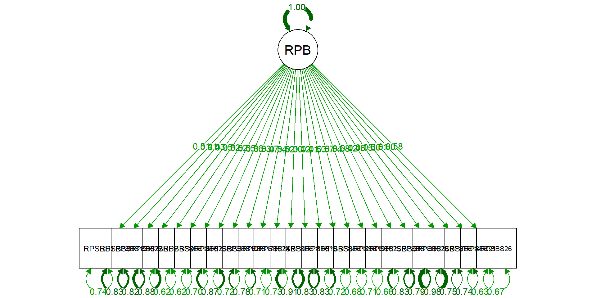
modelR <- 'RPBS     =~ RPSBS1 + RPSBS8 + RPSBS15 + RPSBS22
          + RPSBS2 + RPSBS9 + RPSBS16 + RPSBS23
          + RPSBS3 + RPSBS10 + RPSBS17 + RPSBS24
          + RPSBS4 + RPSBS11 + RPSBS18
          + RPSBS5 + RPSBS12 + RPSBS19 + RPSBS25
          + RPSBS6 + RPSBS13 + RPSBS20
          + RPSBS7 + RPSBS14 + RPSBS21 + RPSBS26'

fitMLRR <- cfa (modelR, std.lv=T, estimator="MLR", data=datRPSBSp)
summary(fitMLRR, standardized=T, modindices = F, fit.measures=T)

lavaan 0.6.16 ended normally after 13 iterations

  Estimator                                         ML
  Optimization method                           NLMINB
  Number of model parameters                        52

  Number of observations                           744

Model Test User Model:
                                              Standard      Scaled
  Test Statistic                               287.168     289.799
  Degrees of freedom                               299         299
  P-value (Chi-square)                           0.678       0.638
  Scaling correction factor                                  0.991
    Yuan-Bentler correction (Mplus variant)                       

Model Test Baseline Model:

  Test statistic                              4080.816    4114.998
  Degrees of freedom                               325         325
  P-value                                        0.000       0.000
  Scaling correction factor                                  0.992

User Model versus Baseline Model:

  Comparative Fit Index (CFI)                    1.000       1.000
  Tucker-Lewis Index (TLI)                       1.003       1.003
                                                                  
  Robust Comparative Fit Index (CFI)                         1.000
  Robust Tucker-Lewis Index (TLI)                            1.003

Loglikelihood and Information Criteria:

  Loglikelihood user model (H0)             -25420.834  -25420.834
  Scaling correction factor                                  1.002
      for the MLR correction                                      
  Loglikelihood unrestricted model (H1)     -25277.250  -25277.250
  Scaling correction factor                                  0.993
      for the MLR correction                                      
                                                                  
  Akaike (AIC)                               50945.669   50945.669
  Bayesian (BIC)                             51185.495   51185.495
  Sample-size adjusted Bayesian (SABIC)      51020.375   51020.375

Root Mean Square Error of Approximation:

  RMSEA                                          0.000       0.000
  90 Percent confidence interval - lower         0.000       0.000
  90 Percent confidence interval - upper         0.012       0.012
  P-value H_0: RMSEA <= 0.050                    1.000       1.000
  P-value H_0: RMSEA >= 0.080                    0.000       0.000
                                                                  
  Robust RMSEA                                               0.000
  90 Percent confidence interval - lower                     0.000
  90 Percent confidence interval - upper                     0.012
  P-value H_0: Robust RMSEA <= 0.050                         1.000
  P-value H_0: Robust RMSEA >= 0.080                         0.000

Standardized Root Mean Square Residual:

  SRMR                                           0.025       0.025

Parameter Estimates:

  Standard errors                             Sandwich
  Information bread                           Observed
  Observed information based on                Hessian

Latent Variables:
                   Estimate  Std.Err  z-value  P(>|z|)   Std.lv  Std.all
  RPBS =~                                                               
    RPSBS1            0.514    0.037   13.815    0.000    0.514    0.514
    RPSBS8            0.405    0.035   11.703    0.000    0.405    0.408
    RPSBS15           0.426    0.037   11.624    0.000    0.426    0.429
    RPSBS22           0.349    0.036    9.781    0.000    0.349    0.351
    RPSBS2            0.607    0.033   18.338    0.000    0.607    0.616
    RPSBS9            0.617    0.036   17.266    0.000    0.617    0.619
    RPSBS16           0.545    0.035   15.387    0.000    0.545    0.548
    RPSBS23           0.364    0.036   10.121    0.000    0.364    0.364
    RPSBS3            0.530    0.036   14.871    0.000    0.530    0.533
    RPSBS10           0.466    0.037   12.562    0.000    0.466    0.469
    RPSBS17           0.527    0.035   15.207    0.000    0.527    0.537
    RPSBS24           0.518    0.035   14.831    0.000    0.518    0.523
    RPSBS4            0.298    0.035    8.412    0.000    0.298    0.298
    RPSBS11           0.407    0.035   11.562    0.000    0.407    0.418
    RPSBS18           0.408    0.036   11.429    0.000    0.408    0.414
    RPSBS5            0.533    0.035   15.069    0.000    0.533    0.533
    RPSBS12           0.566    0.038   14.753    0.000    0.566    0.567
    RPSBS19           0.535    0.034   15.870    0.000    0.535    0.539
    RPSBS25           0.578    0.037   15.540    0.000    0.578    0.582
    RPSBS6            0.414    0.039   10.593    0.000    0.414    0.416
    RPSBS13           0.454    0.034   13.199    0.000    0.454    0.457
    RPSBS20           0.154    0.039    3.978    0.000    0.154    0.154
    RPSBS7            0.498    0.036   13.804    0.000    0.498    0.501
    RPSBS14           0.511    0.036   14.071    0.000    0.511    0.512
    RPSBS21           0.597    0.035   17.294    0.000    0.597    0.604
    RPSBS26           0.576    0.034   16.901    0.000    0.576    0.577

Variances:
                   Estimate  Std.Err  z-value  P(>|z|)   Std.lv  Std.all
   .RPSBS1            0.733    0.039   18.581    0.000    0.733    0.735
   .RPSBS8            0.824    0.049   16.898    0.000    0.824    0.834
   .RPSBS15           0.804    0.040   19.970    0.000    0.804    0.816
   .RPSBS22           0.868    0.041   20.912    0.000    0.868    0.877
   .RPSBS2            0.604    0.034   18.013    0.000    0.604    0.621
   .RPSBS9            0.612    0.035   17.491    0.000    0.612    0.617
   .RPSBS16           0.693    0.038   18.176    0.000    0.693    0.700
   .RPSBS23           0.866    0.044   19.842    0.000    0.866    0.867
   .RPSBS3            0.706    0.038   18.720    0.000    0.706    0.716
   .RPSBS10           0.770    0.040   19.428    0.000    0.770    0.780
   .RPSBS17           0.686    0.034   20.436    0.000    0.686    0.712
   .RPSBS24           0.713    0.038   18.982    0.000    0.713    0.727
   .RPSBS4            0.914    0.044   20.690    0.000    0.914    0.911
   .RPSBS11           0.783    0.043   18.285    0.000    0.783    0.825
   .RPSBS18           0.807    0.045   17.954    0.000    0.807    0.829
   .RPSBS5            0.714    0.038   18.604    0.000    0.714    0.715
   .RPSBS12           0.677    0.039   17.348    0.000    0.677    0.679
   .RPSBS19           0.698    0.039   17.878    0.000    0.698    0.709
   .RPSBS25           0.652    0.037   17.751    0.000    0.652    0.661
   .RPSBS6            0.817    0.045   18.332    0.000    0.817    0.827
   .RPSBS13           0.784    0.039   20.177    0.000    0.784    0.792
   .RPSBS20           0.972    0.051   18.894    0.000    0.972    0.976
   .RPSBS7            0.741    0.042   17.556    0.000    0.741    0.749
   .RPSBS14           0.735    0.040   18.235    0.000    0.735    0.737
   .RPSBS21           0.619    0.035   17.519    0.000    0.619    0.635
   .RPSBS26           0.664    0.037   17.774    0.000    0.664    0.667
    RPBS              1.000                               1.000    1.000

resid(fitMLRR,type="standardized") # Saturations standardisées

$type
[1] "standardized"

$cov
        RPSBS1 RPSBS8 RPSBS15 RPSBS22 RPSBS2 RPSBS9 RPSBS16 RPSBS23 RPSBS3
RPSBS1   0.000                                                            
RPSBS8  -0.247  0.000                                                     
RPSBS15 -1.224 -2.044   0.000                                             
RPSBS22 -0.049 -0.314   0.995   0.000                                     
RPSBS2  -0.070  0.650   0.840   0.523  0.000                              
RPSBS9   0.626  0.023  -1.165  -1.664 -1.414  0.000                       
RPSBS16 -0.166  0.648  -0.343   2.030 -0.104  0.960   0.000               
RPSBS23  1.161  0.086   1.932  -0.719 -0.027 -0.214   1.177   0.000       
RPSBS3   0.101  0.885  -0.573   0.127 -0.685  1.675   0.286  -1.786  0.000
RPSBS10 -0.461 -0.148  -0.051  -0.810 -0.272  2.121  -0.060   0.567 -1.079
RPSBS17  0.126 -1.688  -0.070  -0.935 -0.695 -0.477   1.790   1.798  0.679
RPSBS24 -0.107  1.514   1.421  -1.865 -1.541  0.599  -1.172   0.876 -0.508
RPSBS4   0.127 -0.431  -1.236   1.547 -0.413 -0.529  -1.127  -0.141  1.251
RPSBS11  2.180  0.661  -0.935  -0.159  0.705  0.256  -1.121   0.212  1.283
RPSBS18 -0.451 -0.214   0.108  -0.539  0.035  0.767  -0.235  -2.493  0.185
RPSBS5   1.322 -1.049  -0.284  -0.206  1.835 -0.119   0.568  -0.647 -0.443
RPSBS12 -0.438  0.797   1.992   0.386 -0.168 -0.090   0.723  -0.365 -0.159
RPSBS19 -0.881  1.835  -1.085   1.249 -1.834  0.420   1.790   0.751  0.883
RPSBS25  0.081  0.621  -0.297  -0.331  0.425  0.190   0.038  -1.210 -1.237
RPSBS6   1.073  0.559   1.286   0.287  1.331 -1.366  -0.042  -0.798 -0.911
RPSBS13 -0.823 -1.081  -1.488  -0.239  0.274 -1.310   0.079   0.458 -1.250
RPSBS20  0.179 -0.115  -1.004   0.291 -0.869  0.757   0.017  -0.507  1.031
RPSBS7  -1.092  0.063   0.872  -1.484 -0.752  0.108  -0.408   0.746  0.451
RPSBS14 -1.416 -2.129  -0.072   0.748 -0.503  1.736  -0.539  -0.598  0.001
RPSBS21 -1.165  0.894   2.162   0.948  0.752 -1.444  -2.178  -1.102 -1.100
RPSBS26  2.019 -1.307  -1.279   0.234  1.864 -0.711  -1.948   0.518  1.701
        RPSBS10 RPSBS17 RPSBS24 RPSBS4 RPSBS11 RPSBS18 RPSBS5 RPSBS12 RPSBS19
RPSBS1                                                                       
RPSBS8                                                                       
RPSBS15                                                                      
RPSBS22                                                                      
RPSBS2                                                                       
RPSBS9                                                                       
RPSBS16                                                                      
RPSBS23                                                                      
RPSBS3                                                                       
RPSBS10   0.000                                                              
RPSBS17  -0.031   0.000                                                      
RPSBS24   0.450  -0.701   0.000                                              
RPSBS4    0.545   1.396   0.793  0.000                                       
RPSBS11  -1.546   0.417  -1.403  1.240   0.000                               
RPSBS18  -1.126  -0.299  -0.329  0.455  -1.046   0.000                       
RPSBS5   -0.867  -0.647   1.226 -3.542  -0.337  -0.779  0.000                
RPSBS12   1.268  -0.761  -0.369  0.302   0.941  -0.809 -2.064   0.000        
RPSBS19   0.276  -0.366   0.818  1.570  -0.625   0.709 -0.905   0.000   0.000
RPSBS25   0.467   0.768  -1.381 -0.180  -0.209   0.891  0.198   0.944  -0.400
RPSBS6    1.286  -0.262  -0.535  1.489  -0.436   0.401  0.587  -0.698  -0.496
RPSBS13  -2.329   0.816   1.276 -0.242  -1.026   0.241  1.747  -0.553  -0.113
RPSBS20   0.007  -0.170  -0.857  0.383   0.880  -0.704  0.936   0.313  -0.872
RPSBS7   -0.356   0.740  -0.621 -1.316   0.786   0.512  0.534   0.642   0.871
RPSBS14   0.269  -0.062   1.678  1.286  -0.006   0.972  0.420  -0.844  -0.001
RPSBS21   0.092  -0.719   2.329 -0.757  -0.357   1.243  0.004   0.957  -0.587
RPSBS26   0.352   0.138  -1.694 -0.752  -0.144   0.329  0.803  -1.216  -1.373
        RPSBS25 RPSBS6 RPSBS13 RPSBS20 RPSBS7 RPSBS14 RPSBS21 RPSBS26
RPSBS1                                                               
RPSBS8                                                               
RPSBS15                                                              
RPSBS22                                                              
RPSBS2                                                               
RPSBS9                                                               
RPSBS16                                                              
RPSBS23                                                              
RPSBS3                                                               
RPSBS10                                                              
RPSBS17                                                              
RPSBS24                                                              
RPSBS4                                                               
RPSBS11                                                              
RPSBS18                                                              
RPSBS5                                                               
RPSBS12                                                              
RPSBS19                                                              
RPSBS25   0.000                                                      
RPSBS6   -0.740  0.000                                               
RPSBS13  -1.107  1.229   0.000                                       
RPSBS20   0.320  0.278   0.378   0.000                               
RPSBS7   -0.186 -1.002  -0.306   0.401  0.000                        
RPSBS14  -0.410 -1.295   0.857  -0.003  0.285   0.000                
RPSBS21   1.076  0.239   1.823  -0.397 -1.363   0.158   0.000        
RPSBS26   0.473  0.200   1.719  -0.512  1.394  -0.636  -0.726   0.000

Interprétation des résultats

interpret(fitMLRR) # Intrepréation de la sortie

    Name      Value Threshold Interpretation
1    GFI 0.97148890      0.95   satisfactory
2   AGFI 0.96653045      0.90   satisfactory
3    NFI 0.92962964      0.90   satisfactory
4   NNFI 1.00342412      0.90   satisfactory
5    CFI 1.00000000      0.90   satisfactory
6  RMSEA 0.00000000      0.05   satisfactory
7   SRMR 0.02490191      0.08   satisfactory
8    RFI 0.92351048      0.90   satisfactory
9   PNFI 0.85525927      0.50   satisfactory
10   IFI 1.00312853      0.90   satisfactory

Représentation graphique

Modèle SEM BCB - code

# Modèle en pistes causales

attach(dattotCp)
model0 <- '
  # measurement model
    F_SCSRF =~ SCSRF1 + SCSRF2 + SCSRF3 + SCSRF4 + SCSRF5 + SCSRF6 + SCSRF7 + SCSRF8 + SCSRF9 + SCSRF10
    RPBS    =~ RPSBS1 + RPSBS8 + RPSBS15 + RPSBS22
          + RPSBS2 + RPSBS9 + RPSBS16 + RPSBS23
          + RPSBS3 + RPSBS10 + RPSBS17 + RPSBS24
          + RPSBS4 + RPSBS11 + RPSBS18
          + RPSBS5 + RPSBS12 + RPSBS19 + RPSBS25
          + RPSBS6 + RPSBS13 + RPSBS20
          + RPSBS7 + RPSBS14 + RPSBS21 + RPSBS26
    Eval =~ friendliness + aggressiveness + adopt + emotion
  # regressions
    RPBS ~ F_SCSRF
    Eval ~ RPBS
'

fit0 <- sem(model0, group = "cats", estimator = "mlr", data = dattotCp)
summary(fit0, standardized = TRUE, fit.measures=T)

lavaan 0.6.16 ended normally after 136 iterations

  Estimator                                         ML
  Optimization method                           NLMINB
  Number of model parameters                       244

  Number of observations per group:                   
    B                                              618
    NB                                             121

Model Test User Model:
                                              Standard      Scaled
  Test Statistic                              1672.338    1695.135
  Degrees of freedom                              1476        1476
  P-value (Chi-square)                           0.000       0.000
  Scaling correction factor                                  0.987
    Yuan-Bentler correction (Mplus variant)                       
  Test statistic for each group:
    B                                          772.087     782.612
    NB                                         900.251     912.523

Model Test Baseline Model:

  Test statistic                              7837.331    7920.772
  Degrees of freedom                              1560        1560
  P-value                                        0.000       0.000
  Scaling correction factor                                  0.989

User Model versus Baseline Model:

  Comparative Fit Index (CFI)                    0.969       0.966
  Tucker-Lewis Index (TLI)                       0.967       0.964
                                                                  
  Robust Comparative Fit Index (CFI)                         0.966
  Robust Tucker-Lewis Index (TLI)                            0.964

Loglikelihood and Information Criteria:

  Loglikelihood user model (H0)             -37834.052  -37834.052
  Scaling correction factor                                  1.007
      for the MLR correction                                      
  Loglikelihood unrestricted model (H1)     -36997.883  -36997.883
  Scaling correction factor                                  0.989
      for the MLR correction                                      
                                                                  
  Akaike (AIC)                               76156.104   76156.104
  Bayesian (BIC)                             77279.797   77279.797
  Sample-size adjusted Bayesian (SABIC)      76505.011   76505.011

Root Mean Square Error of Approximation:

  RMSEA                                          0.019       0.020
  90 Percent confidence interval - lower         0.014       0.015
  90 Percent confidence interval - upper         0.023       0.024
  P-value H_0: RMSEA <= 0.050                    1.000       1.000
  P-value H_0: RMSEA >= 0.080                    0.000       0.000
                                                                  
  Robust RMSEA                                               0.020
  90 Percent confidence interval - lower                     0.015
  90 Percent confidence interval - upper                     0.024
  P-value H_0: Robust RMSEA <= 0.050                         1.000
  P-value H_0: Robust RMSEA >= 0.080                         0.000

Standardized Root Mean Square Residual:

  SRMR                                           0.037       0.037

Parameter Estimates:

  Standard errors                             Sandwich
  Information bread                           Observed
  Observed information based on                Hessian


Group 1 [B]:

Latent Variables:
                   Estimate  Std.Err  z-value  P(>|z|)   Std.lv  Std.all
  F_SCSRF =~                                                            
    SCSRF1            1.000                               0.634    0.631
    SCSRF2            1.059    0.086   12.286    0.000    0.671    0.670
    SCSRF3            0.931    0.073   12.716    0.000    0.590    0.608
    SCSRF4            0.998    0.075   13.332    0.000    0.633    0.636
    SCSRF5            0.955    0.070   13.731    0.000    0.605    0.623
    SCSRF6            1.060    0.071   14.993    0.000    0.672    0.680
    SCSRF7            1.032    0.075   13.771    0.000    0.654    0.659
    SCSRF8            0.955    0.074   12.867    0.000    0.605    0.624
    SCSRF9            0.980    0.075   13.012    0.000    0.621    0.628
    SCSRF10           0.936    0.076   12.269    0.000    0.593    0.611
  RPBS =~                                                               
    RPSBS1            1.000                               0.465    0.476
    RPSBS8            0.839    0.103    8.160    0.000    0.390    0.391
    RPSBS15           0.850    0.111    7.672    0.000    0.395    0.394
    RPSBS22           0.769    0.105    7.302    0.000    0.357    0.359
    RPSBS2            1.301    0.132    9.888    0.000    0.605    0.609
    RPSBS9            1.184    0.110   10.788    0.000    0.550    0.579
    RPSBS16           1.095    0.117    9.332    0.000    0.509    0.531
    RPSBS23           0.647    0.094    6.910    0.000    0.301    0.309
    RPSBS3            1.012    0.109    9.294    0.000    0.471    0.492
    RPSBS10           0.939    0.108    8.734    0.000    0.437    0.446
    RPSBS17           1.008    0.107    9.456    0.000    0.469    0.491
    RPSBS24           1.024    0.108    9.484    0.000    0.476    0.492
    RPSBS4            0.531    0.092    5.792    0.000    0.247    0.246
    RPSBS11           0.834    0.101    8.267    0.000    0.387    0.402
    RPSBS18           0.833    0.103    8.091    0.000    0.387    0.394
    RPSBS5            1.081    0.115    9.431    0.000    0.502    0.512
    RPSBS12           1.075    0.113    9.504    0.000    0.500    0.510
    RPSBS19           1.055    0.119    8.876    0.000    0.490    0.502
    RPSBS25           1.190    0.120    9.956    0.000    0.553    0.577
    RPSBS6            0.864    0.112    7.694    0.000    0.402    0.403
    RPSBS13           0.924    0.108    8.592    0.000    0.430    0.441
    RPSBS20           0.315    0.094    3.345    0.001    0.147    0.150
    RPSBS7            1.035    0.123    8.435    0.000    0.481    0.494
    RPSBS14           0.951    0.113    8.425    0.000    0.442    0.464
    RPSBS21           1.297    0.123   10.580    0.000    0.603    0.616
    RPSBS26           1.142    0.112   10.183    0.000    0.531    0.542
  Eval =~                                                               
    friendliness      1.000                               0.342    0.371
    aggressiveness   -1.124    0.201   -5.595    0.000   -0.384   -0.405
    adopt             1.367    0.211    6.477    0.000    0.467    0.493
    emotion           1.173    0.198    5.934    0.000    0.401    0.426

Regressions:
                   Estimate  Std.Err  z-value  P(>|z|)   Std.lv  Std.all
  RPBS ~                                                                
    F_SCSRF           0.430    0.052    8.352    0.000    0.587    0.587
  Eval ~                                                                
    RPBS             -0.629    0.089   -7.109    0.000   -0.856   -0.856

Intercepts:
                   Estimate  Std.Err  z-value  P(>|z|)   Std.lv  Std.all
   .SCSRF1            0.066    0.040    1.634    0.102    0.066    0.066
   .SCSRF2            0.079    0.040    1.949    0.051    0.079    0.078
   .SCSRF3            0.068    0.039    1.751    0.080    0.068    0.070
   .SCSRF4            0.090    0.040    2.255    0.024    0.090    0.091
   .SCSRF5            0.060    0.039    1.526    0.127    0.060    0.061
   .SCSRF6            0.064    0.040    1.609    0.108    0.064    0.065
   .SCSRF7            0.088    0.040    2.215    0.027    0.088    0.089
   .SCSRF8            0.059    0.039    1.509    0.131    0.059    0.061
   .SCSRF9            0.074    0.040    1.866    0.062    0.074    0.075
   .SCSRF10           0.065    0.039    1.668    0.095    0.065    0.067
   .RPSBS1            0.089    0.039    2.273    0.023    0.089    0.091
   .RPSBS8            0.067    0.040    1.678    0.093    0.067    0.067
   .RPSBS15           0.091    0.040    2.258    0.024    0.091    0.091
   .RPSBS22           0.062    0.040    1.546    0.122    0.062    0.062
   .RPSBS2            0.080    0.040    1.994    0.046    0.080    0.080
   .RPSBS9            0.111    0.038    2.896    0.004    0.111    0.117
   .RPSBS16           0.110    0.039    2.859    0.004    0.110    0.115
   .RPSBS23           0.073    0.039    1.873    0.061    0.073    0.075
   .RPSBS3            0.089    0.039    2.301    0.021    0.089    0.093
   .RPSBS10           0.066    0.039    1.689    0.091    0.066    0.068
   .RPSBS17           0.083    0.038    2.172    0.030    0.083    0.087
   .RPSBS24           0.074    0.039    1.910    0.056    0.074    0.077
   .RPSBS4            0.059    0.040    1.467    0.142    0.059    0.059
   .RPSBS11           0.058    0.039    1.484    0.138    0.058    0.060
   .RPSBS18           0.060    0.039    1.510    0.131    0.060    0.061
   .RPSBS5            0.070    0.039    1.769    0.077    0.070    0.071
   .RPSBS12           0.113    0.039    2.861    0.004    0.113    0.115
   .RPSBS19           0.106    0.039    2.683    0.007    0.106    0.108
   .RPSBS25           0.100    0.039    2.600    0.009    0.100    0.105
   .RPSBS6            0.078    0.040    1.944    0.052    0.078    0.078
   .RPSBS13           0.060    0.039    1.523    0.128    0.060    0.061
   .RPSBS20           0.016    0.039    0.408    0.683    0.016    0.016
   .RPSBS7            0.077    0.039    1.954    0.051    0.077    0.079
   .RPSBS14           0.100    0.038    2.616    0.009    0.100    0.105
   .RPSBS21           0.094    0.039    2.377    0.017    0.094    0.096
   .RPSBS26           0.088    0.039    2.244    0.025    0.088    0.090
   .friendliness     -0.202    0.037   -5.448    0.000   -0.202   -0.219
   .aggressiveness    0.192    0.038    5.034    0.000    0.192    0.202
   .adopt            -0.182    0.038   -4.768    0.000   -0.182   -0.192
   .emotion          -0.183    0.038   -4.834    0.000   -0.183   -0.194
    F_SCSRF           0.000                               0.000    0.000
   .RPBS              0.000                               0.000    0.000
   .Eval              0.000                               0.000    0.000

Variances:
                   Estimate  Std.Err  z-value  P(>|z|)   Std.lv  Std.all
   .SCSRF1            0.607    0.038   16.021    0.000    0.607    0.602
   .SCSRF2            0.553    0.034   16.281    0.000    0.553    0.551
   .SCSRF3            0.595    0.033   18.224    0.000    0.595    0.631
   .SCSRF4            0.590    0.037   16.168    0.000    0.590    0.596
   .SCSRF5            0.577    0.035   16.703    0.000    0.577    0.612
   .SCSRF6            0.525    0.033   15.672    0.000    0.525    0.537
   .SCSRF7            0.559    0.038   14.716    0.000    0.559    0.566
   .SCSRF8            0.575    0.032   17.924    0.000    0.575    0.611
   .SCSRF9            0.592    0.038   15.617    0.000    0.592    0.605
   .SCSRF10           0.589    0.035   17.045    0.000    0.589    0.626
   .RPSBS1            0.737    0.043   17.097    0.000    0.737    0.773
   .RPSBS8            0.841    0.056   15.052    0.000    0.841    0.847
   .RPSBS15           0.848    0.045   18.774    0.000    0.848    0.845
   .RPSBS22           0.866    0.047   18.595    0.000    0.866    0.871
   .RPSBS2            0.622    0.037   16.782    0.000    0.622    0.630
   .RPSBS9            0.601    0.036   16.475    0.000    0.601    0.665
   .RPSBS16           0.660    0.039   16.722    0.000    0.660    0.718
   .RPSBS23           0.854    0.048   17.849    0.000    0.854    0.904
   .RPSBS3            0.695    0.041   17.106    0.000    0.695    0.758
   .RPSBS10           0.766    0.043   17.616    0.000    0.766    0.801
   .RPSBS17           0.690    0.037   18.674    0.000    0.690    0.759
   .RPSBS24           0.708    0.041   17.259    0.000    0.708    0.758
   .RPSBS4            0.943    0.050   18.788    0.000    0.943    0.939
   .RPSBS11           0.778    0.045   17.157    0.000    0.778    0.838
   .RPSBS18           0.814    0.050   16.211    0.000    0.814    0.845
   .RPSBS5            0.709    0.042   16.832    0.000    0.709    0.738
   .RPSBS12           0.710    0.043   16.361    0.000    0.710    0.740
   .RPSBS19           0.715    0.044   16.382    0.000    0.715    0.748
   .RPSBS25           0.614    0.037   16.640    0.000    0.614    0.667
   .RPSBS6            0.830    0.051   16.371    0.000    0.830    0.837
   .RPSBS13           0.766    0.042   18.463    0.000    0.766    0.806
   .RPSBS20           0.940    0.054   17.507    0.000    0.940    0.978
   .RPSBS7            0.718    0.043   16.595    0.000    0.718    0.756
   .RPSBS14           0.712    0.041   17.260    0.000    0.712    0.785
   .RPSBS21           0.596    0.036   16.335    0.000    0.596    0.621
   .RPSBS26           0.677    0.040   16.831    0.000    0.677    0.706
   .friendliness      0.731    0.044   16.620    0.000    0.731    0.862
   .aggressiveness    0.754    0.041   18.395    0.000    0.754    0.836
   .adopt             0.681    0.047   14.609    0.000    0.681    0.757
   .emotion           0.724    0.043   16.898    0.000    0.724    0.818
    F_SCSRF           0.402    0.048    8.346    0.000    1.000    1.000
   .RPBS              0.142    0.023    6.051    0.000    0.656    0.656
   .Eval              0.031    0.013    2.486    0.013    0.268    0.268


Group 2 [NB]:

Latent Variables:
                   Estimate  Std.Err  z-value  P(>|z|)   Std.lv  Std.all
  F_SCSRF =~                                                            
    SCSRF1            1.000                               0.550    0.603
    SCSRF2            1.058    0.164    6.448    0.000    0.582    0.665
    SCSRF3            1.162    0.231    5.034    0.000    0.639    0.602
    SCSRF4            0.905    0.183    4.931    0.000    0.497    0.558
    SCSRF5            1.053    0.203    5.192    0.000    0.579    0.574
    SCSRF6            1.203    0.180    6.685    0.000    0.661    0.672
    SCSRF7            0.969    0.185    5.250    0.000    0.532    0.581
    SCSRF8            1.401    0.223    6.281    0.000    0.770    0.725
    SCSRF9            1.069    0.167    6.393    0.000    0.588    0.641
    SCSRF10           1.269    0.214    5.936    0.000    0.698    0.648
  RPBS =~                                                               
    RPSBS1            1.000                               0.541    0.551
    RPSBS8            0.674    0.161    4.195    0.000    0.365    0.393
    RPSBS15           0.473    0.160    2.960    0.003    0.256    0.315
    RPSBS22           0.156    0.153    1.020    0.308    0.085    0.094
    RPSBS2            0.966    0.194    4.980    0.000    0.522    0.591
    RPSBS9            1.127    0.264    4.265    0.000    0.609    0.605
    RPSBS16           0.776    0.187    4.154    0.000    0.419    0.421
    RPSBS23           1.046    0.199    5.244    0.000    0.566    0.535
    RPSBS3            0.961    0.226    4.248    0.000    0.519    0.515
    RPSBS10           0.726    0.210    3.451    0.001    0.392    0.400
    RPSBS17           0.981    0.201    4.880    0.000    0.530    0.539
    RPSBS24           0.957    0.221    4.323    0.000    0.517    0.529
    RPSBS4            0.563    0.189    2.972    0.003    0.304    0.325
    RPSBS11           0.650    0.181    3.591    0.000    0.352    0.381
    RPSBS18           0.597    0.207    2.889    0.004    0.323    0.339
    RPSBS5            0.950    0.221    4.295    0.000    0.513    0.511
    RPSBS12           0.907    0.189    4.795    0.000    0.490    0.548
    RPSBS19           0.914    0.184    4.969    0.000    0.494    0.546
    RPSBS25           0.944    0.207    4.562    0.000    0.510    0.501
    RPSBS6            0.537    0.193    2.777    0.005    0.290    0.322
    RPSBS13           0.931    0.221    4.202    0.000    0.503    0.503
    RPSBS20           0.297    0.201    1.480    0.139    0.161    0.149
    RPSBS7            0.754    0.206    3.662    0.000    0.407    0.409
    RPSBS14           0.890    0.244    3.650    0.000    0.481    0.487
    RPSBS21           0.824    0.200    4.117    0.000    0.446    0.493
    RPSBS26           1.191    0.214    5.567    0.000    0.644    0.662
  Eval =~                                                               
    friendliness      1.000                               0.178    0.275
    aggressiveness   -1.296    1.312   -0.988    0.323   -0.230   -0.382
    adopt             1.058    0.897    1.179    0.238    0.188    0.328
    emotion           1.938    1.697    1.142    0.253    0.344    0.494

Regressions:
                   Estimate  Std.Err  z-value  P(>|z|)   Std.lv  Std.all
  RPBS ~                                                                
    F_SCSRF           0.484    0.134    3.600    0.000    0.492    0.492
  Eval ~                                                                
    RPBS             -0.251    0.209   -1.202    0.229   -0.764   -0.764

Intercepts:
                   Estimate  Std.Err  z-value  P(>|z|)   Std.lv  Std.all
   .SCSRF1           -0.281    0.083   -3.395    0.001   -0.281   -0.309
   .SCSRF2           -0.399    0.079   -5.021    0.000   -0.399   -0.456
   .SCSRF3           -0.370    0.096   -3.839    0.000   -0.370   -0.349
   .SCSRF4           -0.437    0.081   -5.396    0.000   -0.437   -0.491
   .SCSRF5           -0.284    0.092   -3.099    0.002   -0.284   -0.282
   .SCSRF6           -0.328    0.089   -3.666    0.000   -0.328   -0.333
   .SCSRF7           -0.427    0.083   -5.130    0.000   -0.427   -0.466
   .SCSRF8           -0.292    0.097   -3.028    0.002   -0.292   -0.275
   .SCSRF9           -0.391    0.083   -4.697    0.000   -0.391   -0.427
   .SCSRF10          -0.324    0.098   -3.311    0.001   -0.324   -0.301
   .RPSBS1           -0.439    0.089   -4.920    0.000   -0.439   -0.447
   .RPSBS8           -0.315    0.084   -3.736    0.000   -0.315   -0.340
   .RPSBS15          -0.465    0.074   -6.302    0.000   -0.465   -0.573
   .RPSBS22          -0.320    0.082   -3.913    0.000   -0.320   -0.356
   .RPSBS2           -0.396    0.080   -4.929    0.000   -0.396   -0.448
   .RPSBS9           -0.584    0.091   -6.391    0.000   -0.584   -0.581
   .RPSBS16          -0.562    0.091   -6.204    0.000   -0.562   -0.564
   .RPSBS23          -0.335    0.096   -3.484    0.000   -0.335   -0.317
   .RPSBS3           -0.492    0.092   -5.371    0.000   -0.492   -0.488
   .RPSBS10          -0.325    0.089   -3.652    0.000   -0.325   -0.332
   .RPSBS17          -0.467    0.089   -5.226    0.000   -0.467   -0.475
   .RPSBS24          -0.390    0.089   -4.386    0.000   -0.390   -0.399
   .RPSBS4           -0.314    0.085   -3.691    0.000   -0.314   -0.336
   .RPSBS11          -0.324    0.084   -3.853    0.000   -0.324   -0.350
   .RPSBS18          -0.310    0.087   -3.583    0.000   -0.310   -0.326
   .RPSBS5           -0.391    0.091   -4.281    0.000   -0.391   -0.389
   .RPSBS12          -0.564    0.081   -6.939    0.000   -0.564   -0.631
   .RPSBS19          -0.529    0.082   -6.428    0.000   -0.529   -0.584
   .RPSBS25          -0.477    0.093   -5.148    0.000   -0.477   -0.468
   .RPSBS6           -0.337    0.082   -4.106    0.000   -0.337   -0.373
   .RPSBS13          -0.302    0.091   -3.328    0.001   -0.302   -0.303
   .RPSBS20          -0.071    0.098   -0.728    0.467   -0.071   -0.066
   .RPSBS7           -0.410    0.091   -4.529    0.000   -0.410   -0.412
   .RPSBS14          -0.553    0.090   -6.161    0.000   -0.553   -0.560
   .RPSBS21          -0.439    0.082   -5.343    0.000   -0.439   -0.486
   .RPSBS26          -0.428    0.088   -4.847    0.000   -0.428   -0.441
   .friendliness      1.041    0.059   17.719    0.000    1.041    1.611
   .aggressiveness   -0.926    0.055  -16.923    0.000   -0.926   -1.538
   .adopt             0.949    0.052   18.195    0.000    0.949    1.654
   .emotion           0.927    0.063   14.644    0.000    0.927    1.331
    F_SCSRF           0.000                               0.000    0.000
   .RPBS              0.000                               0.000    0.000
   .Eval              0.000                               0.000    0.000

Variances:
                   Estimate  Std.Err  z-value  P(>|z|)   Std.lv  Std.all
   .SCSRF1            0.529    0.078    6.799    0.000    0.529    0.637
   .SCSRF2            0.426    0.060    7.163    0.000    0.426    0.558
   .SCSRF3            0.717    0.096    7.479    0.000    0.717    0.637
   .SCSRF4            0.546    0.075    7.286    0.000    0.546    0.688
   .SCSRF5            0.682    0.095    7.212    0.000    0.682    0.671
   .SCSRF6            0.530    0.072    7.353    0.000    0.530    0.548
   .SCSRF7            0.556    0.080    6.953    0.000    0.556    0.663
   .SCSRF8            0.535    0.084    6.344    0.000    0.535    0.474
   .SCSRF9            0.495    0.077    6.421    0.000    0.495    0.589
   .SCSRF10           0.673    0.095    7.061    0.000    0.673    0.580
   .RPSBS1            0.670    0.088    7.625    0.000    0.670    0.696
   .RPSBS8            0.725    0.094    7.724    0.000    0.725    0.845
   .RPSBS15           0.593    0.079    7.475    0.000    0.593    0.901
   .RPSBS22           0.802    0.080   10.024    0.000    0.802    0.991
   .RPSBS2            0.508    0.073    6.939    0.000    0.508    0.651
   .RPSBS9            0.641    0.101    6.369    0.000    0.641    0.633
   .RPSBS16           0.817    0.099    8.225    0.000    0.817    0.823
   .RPSBS23           0.799    0.100    7.964    0.000    0.799    0.714
   .RPSBS3            0.747    0.092    8.071    0.000    0.747    0.735
   .RPSBS10           0.807    0.103    7.801    0.000    0.807    0.840
   .RPSBS17           0.687    0.076    9.046    0.000    0.687    0.710
   .RPSBS24           0.688    0.080    8.574    0.000    0.688    0.720
   .RPSBS4            0.785    0.093    8.468    0.000    0.785    0.894
   .RPSBS11           0.730    0.091    8.020    0.000    0.730    0.855
   .RPSBS18           0.804    0.104    7.750    0.000    0.804    0.885
   .RPSBS5            0.745    0.096    7.755    0.000    0.745    0.739
   .RPSBS12           0.560    0.077    7.266    0.000    0.560    0.700
   .RPSBS19           0.575    0.080    7.231    0.000    0.575    0.702
   .RPSBS25           0.778    0.098    7.963    0.000    0.778    0.749
   .RPSBS6            0.730    0.083    8.771    0.000    0.730    0.897
   .RPSBS13           0.746    0.092    8.152    0.000    0.746    0.747
   .RPSBS20           1.137    0.157    7.225    0.000    1.137    0.978
   .RPSBS7            0.826    0.129    6.392    0.000    0.826    0.833
   .RPSBS14           0.743    0.099    7.534    0.000    0.743    0.762
   .RPSBS21           0.619    0.087    7.155    0.000    0.619    0.757
   .RPSBS26           0.530    0.096    5.524    0.000    0.530    0.561
   .friendliness      0.386    0.061    6.321    0.000    0.386    0.925
   .aggressiveness    0.310    0.066    4.710    0.000    0.310    0.854
   .adopt             0.294    0.039    7.609    0.000    0.294    0.893
   .emotion           0.367    0.099    3.708    0.000    0.367    0.756
    F_SCSRF           0.302    0.077    3.908    0.000    1.000    1.000
   .RPBS              0.221    0.080    2.766    0.006    0.758    0.758
   .Eval              0.013    0.010    1.318    0.187    0.416    0.416

Le modèle s’ajuste aux données ?

interpret(fit0) # Intrepréation de la sortie

    Name      Value Threshold Interpretation
1    GFI 0.92026518      0.95           poor
2   AGFI 0.90708409      0.90   satisfactory
3    NFI 0.78661901      0.90           poor
4   NNFI 0.96694276      0.90   satisfactory
5    CFI 0.96872277      0.90   satisfactory
6  RMSEA 0.01897367      0.05   satisfactory
7   SRMR 0.03745996      0.08   satisfactory
8    RFI 0.77447537      0.90           poor
9   PNFI 0.74426260      0.50   satisfactory
10   IFI 0.96913578      0.90   satisfactory

Modèle SEM BCB - résultats

Regression parameters from `path analysis`
Term	estimate	z	p
RPBS ~ F_SCSRF	0.4303	8.352	0
Eval ~ RPBS	-0.6294	-7.109	1.168e-12
RPBS ~ F_SCSRF	0.4839	3.6	0.0003185
Eval ~ RPBS	-0.251	-1.202	0.2292

Modèle SEM BCB - résultats

Les SEM - Méthode de régression médiations / modérations

Exemple : La beauté réside dans les yeux du buveur de bières

Beauty is in the eye of the beer holder

Modèle de régression

Effet médiateur

Médiation modèle de Baron & Kenny (1986)

Modèle Baron et Kenny étape 1

Y<---X

# 4 étapes de médiation - Baron et Kenny (1986)
# Etape 1 - R?gression lin?aire simple VD ~ VI

model01<-lm(DF$Att~DF$BALlog)
summary(model01)


Call:
lm(formula = DF$Att ~ DF$BALlog)

Residuals:
    Min      1Q  Median      3Q     Max 
-2.7274 -0.7684 -0.0068  0.7278  3.2412 

Coefficients:
            Estimate Std. Error t value Pr(>|t|)  
(Intercept) -17.1500    26.5967  -0.645   0.5193  
DF$BALlog     0.9016     0.4586   1.966   0.0498 *
---
Signif. codes:  0 '***' 0.001 '**' 0.01 '*' 0.05 '.' 0.1 ' ' 1

Residual standard error: 1.06 on 498 degrees of freedom
Multiple R-squared:  0.007703,  Adjusted R-squared:  0.005711 
F-statistic: 3.866 on 1 and 498 DF,  p-value: 0.04983

Modèle de Baron et Kenny étape 2

M<---X

# Etape 2 - Régression logistique (VM : catégoriel) simple VM ~ VI

model02<-glm(factor(DF$Expect_dummy)~DF$BALlog, family = binomial)
summary(model02, Wald = TRUE)


Call:
glm(formula = factor(DF$Expect_dummy) ~ DF$BALlog, family = binomial)

Coefficients:
            Estimate Std. Error z value Pr(>|z|)    
(Intercept) -592.247     68.850  -8.602   <2e-16 ***
DF$BALlog     10.214      1.187   8.603   <2e-16 ***
---
Signif. codes:  0 '***' 0.001 '**' 0.01 '*' 0.05 '.' 0.1 ' ' 1

(Dispersion parameter for binomial family taken to be 1)

    Null deviance: 691.10  on 499  degrees of freedom
Residual deviance: 591.63  on 498  degrees of freedom
AIC: 595.63

Number of Fisher Scoring iterations: 4

confint(model02, level = 0.95)

                  2.5 %     97.5 %
(Intercept) -732.131206 -461.85054
DF$BALlog      7.965496   12.62601

Modèle de Baron et Kenny étape 3 & 4

Y<---M+X

model34<-lm(DF$Att~factor(DF$Expect_dummy) + DF$BALlog)
summary(model34)


Call:
lm(formula = DF$Att ~ factor(DF$Expect_dummy) + DF$BALlog)

Residuals:
     Min       1Q   Median       3Q      Max 
-2.75045 -0.65655 -0.02656  0.67795  2.78261 

Coefficients:
                         Estimate Std. Error t value Pr(>|t|)    
(Intercept)              84.66438   27.27528   3.104  0.00202 ** 
factor(DF$Expect_dummy)1  0.86439    0.09751   8.865  < 2e-16 ***
DF$BALlog                -0.86170    0.47064  -1.831  0.06771 .  
---
Signif. codes:  0 '***' 0.001 '**' 0.01 '*' 0.05 '.' 0.1 ' ' 1

Residual standard error: 0.986 on 497 degrees of freedom
Multiple R-squared:  0.1432,    Adjusted R-squared:  0.1397 
F-statistic: 41.53 on 2 and 497 DF,  p-value: < 2.2e-16

Modèle SEM - 1 médiateur

Modèle SEM BEBH - code

attach(DF)
model01<-'#
        Att ~ Expect_dummy + BALlog
        Expect_dummy ~ BALlog'

fit01<-sem(model01, data=DF, estimator="DWLS")
summary(fit01, fit.measures=T, rsquare=T, standardized = T)

lavaan 0.6.16 ended normally after 1 iteration

  Estimator                                       DWLS
  Optimization method                           NLMINB
  Number of model parameters                         6

  Number of observations                           500

Model Test User Model:
                                                      
  Test statistic                                 0.000
  Degrees of freedom                                 0

Model Test Baseline Model:

  Test statistic                               192.268
  Degrees of freedom                                 3
  P-value                                        0.000

User Model versus Baseline Model:

  Comparative Fit Index (CFI)                    1.000
  Tucker-Lewis Index (TLI)                       1.000

Root Mean Square Error of Approximation:

  RMSEA                                          0.000
  90 Percent confidence interval - lower         0.000
  90 Percent confidence interval - upper         0.000
  P-value H_0: RMSEA <= 0.050                       NA
  P-value H_0: RMSEA >= 0.080                       NA

Standardized Root Mean Square Residual:

  SRMR                                           0.000

Parameter Estimates:

  Standard errors                             Standard
  Information                                 Expected
  Information saturated (h1) model        Unstructured

Regressions:
                   Estimate  Std.Err  z-value  P(>|z|)   Std.lv  Std.all
  Att ~                                                                 
    Expect_dummy      0.864    0.121    7.150    0.000    0.864    0.406
    BALlog           -0.862    0.635   -1.358    0.174   -0.862   -0.084
  Expect_dummy ~                                                        
    BALlog            2.040    0.239    8.536    0.000    2.040    0.423

Variances:
                   Estimate  Std.Err  z-value  P(>|z|)   Std.lv  Std.all
   .Att               0.968    0.076   12.776    0.000    0.968    0.857
   .Expect_dummy      0.205    0.009   22.308    0.000    0.205    0.821
    BALlog            0.011    0.001   14.945    0.000    0.011    1.000

R-Square:
                   Estimate
    Att               0.143
    Expect_dummy      0.179

Modèle SEM BEBH - code

attach(DF)
model<-'#direct effect
        Att ~ c*BALlog
        #mediator
        Expect_dummy ~ a*BALlog
        Att ~ b*Expect_dummy
        #Indirect effect (a*b)
        ab := a*b
        # Total Effect
        total := c + (a*b)'

fit<-sem(model, data=DF, estimator="MLR") # Méthode robuste fonctionne aussi sur données catégorielles
summary(fit, fit.measures=T, rsquare=T, standardized = T)

lavaan 0.6.16 ended normally after 1 iteration

  Estimator                                         ML
  Optimization method                           NLMINB
  Number of model parameters                         5

  Number of observations                           500

Model Test User Model:
                                              Standard      Scaled
  Test Statistic                                 0.000       0.000
  Degrees of freedom                                 0           0

Model Test Baseline Model:

  Test statistic                               175.656     169.920
  Degrees of freedom                                 3           3
  P-value                                        0.000       0.000
  Scaling correction factor                                  1.034

User Model versus Baseline Model:

  Comparative Fit Index (CFI)                    1.000       1.000
  Tucker-Lewis Index (TLI)                       1.000       1.000
                                                                  
  Robust Comparative Fit Index (CFI)                            NA
  Robust Tucker-Lewis Index (TLI)                               NA

Loglikelihood and Information Criteria:

  Loglikelihood user model (H0)              -1013.582   -1013.582
  Loglikelihood unrestricted model (H1)      -1013.582   -1013.582
                                                                  
  Akaike (AIC)                                2037.164    2037.164
  Bayesian (BIC)                              2058.237    2058.237
  Sample-size adjusted Bayesian (SABIC)       2042.367    2042.367

Root Mean Square Error of Approximation:

  RMSEA                                          0.000          NA
  90 Percent confidence interval - lower         0.000          NA
  90 Percent confidence interval - upper         0.000          NA
  P-value H_0: RMSEA <= 0.050                       NA          NA
  P-value H_0: RMSEA >= 0.080                       NA          NA
                                                                  
  Robust RMSEA                                               0.000
  90 Percent confidence interval - lower                     0.000
  90 Percent confidence interval - upper                     0.000
  P-value H_0: Robust RMSEA <= 0.050                            NA
  P-value H_0: Robust RMSEA >= 0.080                            NA

Standardized Root Mean Square Residual:

  SRMR                                           0.000       0.000

Parameter Estimates:

  Standard errors                             Sandwich
  Information bread                           Observed
  Observed information based on                Hessian

Regressions:
                   Estimate  Std.Err  z-value  P(>|z|)   Std.lv  Std.all
  Att ~                                                                 
    BALlog     (c)   -0.862    0.447   -1.926    0.054   -0.862   -0.084
  Expect_dummy ~                                                        
    BALlog     (a)    2.040    0.176   11.602    0.000    2.040    0.423
  Att ~                                                                 
    Expct_dmmy (b)    0.864    0.094    9.157    0.000    0.864    0.406

Variances:
                   Estimate  Std.Err  z-value  P(>|z|)   Std.lv  Std.all
   .Att               0.966    0.057   16.849    0.000    0.966    0.857
   .Expect_dummy      0.205    0.008   26.850    0.000    0.205    0.821

R-Square:
                   Estimate
    Att               0.143
    Expect_dummy      0.179

Defined Parameters:
                   Estimate  Std.Err  z-value  P(>|z|)   Std.lv  Std.all
    ab                1.763    0.239    7.393    0.000    1.763    0.172
    total             0.902    0.447    2.016    0.044    0.902    0.088

Modèle SEM BEBH - Ajustement du modèle aux données

interpret(fit) # Intrepréation de la sortie

    Name        Value Threshold Interpretation
1    GFI 1.000000e+00      0.95   satisfactory
2   AGFI 1.000000e+00      0.90   satisfactory
3    NFI 1.000000e+00      0.90   satisfactory
4   NNFI 1.000000e+00      0.90   satisfactory
5    CFI 1.000000e+00      0.90   satisfactory
6  RMSEA 0.000000e+00      0.05   satisfactory
7   SRMR 5.099025e-17      0.08   satisfactory
8    RFI 1.000000e+00      0.90   satisfactory
9   PNFI 0.000000e+00      0.50           poor
10   IFI 1.000000e+00      0.90   satisfactory

Modèle SEM BEBH - résultats

Regression parameters from `mediation` (continued below)
lhs	op	rhs	label	estimate	se	z
Att	~	BALlog	c	-0.8617	0.4473	-1.926
Expect_dummy	~	BALlog	a	2.04	0.1758	11.6
Att	~	Expect_dummy	b	0.8644	0.09439	9.157

p	ci.lower	ci.upper	Term
0.05407	-1.738	0.01508	Att ~ BALlog
0	1.695	2.385	Expect_dummy ~ BALlog
0	0.6794	1.049	Att ~ Expect_dummy

Modèle SEM BEBH - représentation graphique

graph1<-semPlot::semPaths(fit, "par",
             sizeMan = 10, sizeInt = 10, sizeLat = 10,
             edge.label.cex=1.5,
             fade=FALSE)

Modèle SEM BEBH - représentation graphique avec étoiles

graph_stars <- mark_sig(graph1, fit)
plot(graph_stars)

Modèle SEM 2 médiateurs

Modèle SEM 2 médiateurs - code

attach(DF2)
model2<-'#direct effect
        Att ~ c*BALlog
        #mediator
        Expect_dummy ~ a1*BALlog
        EdS ~ a2*BALlog
        Att ~ b1*Expect_dummy
        Att ~ b2*EdS
        #Indirect effect (a*b)
        ab1 := a1*b1
        ab2 := a2*b2
        # Total Effect
        total := c + (a1*b1) + (a2*b2)
        Expect_dummy~~EdS'

fit2<-sem(model2, data=DF2, estimator="MLR")
summary(fit2, fit.measures=T, rsquare=T, standardized = T)

lavaan 0.6.16 ended normally after 12 iterations

  Estimator                                         ML
  Optimization method                           NLMINB
  Number of model parameters                         9

  Number of observations                           500

Model Test User Model:
                                              Standard      Scaled
  Test Statistic                                 0.000       0.000
  Degrees of freedom                                 0           0

Model Test Baseline Model:

  Test statistic                               313.840     323.946
  Degrees of freedom                                 6           6
  P-value                                        0.000       0.000
  Scaling correction factor                                  0.969

User Model versus Baseline Model:

  Comparative Fit Index (CFI)                    1.000       1.000
  Tucker-Lewis Index (TLI)                       1.000       1.000
                                                                  
  Robust Comparative Fit Index (CFI)                            NA
  Robust Tucker-Lewis Index (TLI)                               NA

Loglikelihood and Information Criteria:

  Loglikelihood user model (H0)              -1714.216   -1714.216
  Loglikelihood unrestricted model (H1)      -1714.216   -1714.216
                                                                  
  Akaike (AIC)                                3446.431    3446.431
  Bayesian (BIC)                              3484.363    3484.363
  Sample-size adjusted Bayesian (SABIC)       3455.796    3455.796

Root Mean Square Error of Approximation:

  RMSEA                                          0.000          NA
  90 Percent confidence interval - lower         0.000          NA
  90 Percent confidence interval - upper         0.000          NA
  P-value H_0: RMSEA <= 0.050                       NA          NA
  P-value H_0: RMSEA >= 0.080                       NA          NA
                                                                  
  Robust RMSEA                                               0.000
  90 Percent confidence interval - lower                     0.000
  90 Percent confidence interval - upper                     0.000
  P-value H_0: Robust RMSEA <= 0.050                            NA
  P-value H_0: Robust RMSEA >= 0.080                            NA

Standardized Root Mean Square Residual:

  SRMR                                           0.000       0.000

Parameter Estimates:

  Standard errors                             Sandwich
  Information bread                           Observed
  Observed information based on                Hessian

Regressions:
                   Estimate  Std.Err  z-value  P(>|z|)   Std.lv  Std.all
  Att ~                                                                 
    BALlog     (c)   -0.938    0.441   -2.128    0.033   -0.938   -0.077
  Expect_dummy ~                                                        
    BALlog    (a1)    2.040    0.176   11.602    0.000    2.040    0.423
  EdS ~                                                                 
    BALlog    (a2)    0.144    0.399    0.362    0.717    0.144    0.016
  Att ~                                                                 
    Expct_dmm (b1)    0.828    0.097    8.504    0.000    0.828    0.330
    EdS       (b2)   -0.667    0.048  -13.951    0.000   -0.667   -0.509

Covariances:
                   Estimate  Std.Err  z-value  P(>|z|)   Std.lv  Std.all
 .Expect_dummy ~~                                                       
   .EdS               0.001    0.019    0.074    0.941    0.001    0.003

Variances:
                   Estimate  Std.Err  z-value  P(>|z|)   Std.lv  Std.all
   .Att               1.021    0.063   16.316    0.000    1.021    0.650
   .Expect_dummy      0.205    0.008   26.850    0.000    0.205    0.821
   .EdS               0.914    0.058   15.636    0.000    0.914    1.000

R-Square:
                   Estimate
    Att               0.350
    Expect_dummy      0.179
    EdS               0.000

Defined Parameters:
                   Estimate  Std.Err  z-value  P(>|z|)   Std.lv  Std.all
    ab1               1.690    0.241    7.004    0.000    1.690    0.139
    ab2              -0.096    0.266   -0.361    0.718   -0.096   -0.008
    total             0.656    0.529    1.241    0.214    0.656    0.054

Modèle SEM 2 médiateurs - Ajustement aux données

interpret(fit2) # Intrepréation de la sortie

    Name        Value Threshold Interpretation
1    GFI 1.000000e+00      0.95   satisfactory
2   AGFI 1.000000e+00      0.90   satisfactory
3    NFI 1.000000e+00      0.90   satisfactory
4   NNFI 1.000000e+00      0.90   satisfactory
5    CFI 1.000000e+00      0.90   satisfactory
6  RMSEA 0.000000e+00      0.05   satisfactory
7   SRMR 2.525178e-08      0.08   satisfactory
8    RFI 1.000000e+00      0.90   satisfactory
9   PNFI 0.000000e+00      0.50           poor
10   IFI 1.000000e+00      0.90   satisfactory

Modèle SEM 2 médiateurs - résultats

Regression parameters from `mediation 2` (continued below)
lhs	op	rhs	label	estimate	se	z
Att	~	BALlog	c	-0.9378	0.4406	-2.128
Expect_dummy	~	BALlog	a1	2.04	0.1758	11.6
EdS	~	BALlog	a2	0.1443	0.3988	0.3619
Att	~	Expect_dummy	b1	0.8285	0.09742	8.504
Att	~	EdS	b2	-0.6666	0.04778	-13.95

p	ci.lower	ci.upper	Term
0.03332	-1.801	-0.07413	Att ~ BALlog
0	1.695	2.385	Expect_dummy ~ BALlog
0.7175	-0.6374	0.926	EdS ~ BALlog
0	0.6375	1.019	Att ~ Expect_dummy
0	-0.7602	-0.5729	Att ~ EdS

Modèle SEM 2 médiateurs - représentation graphique

semPlot::semPaths(fit2, "par",
             sizeMan = 10, sizeInt = 10, sizeLat = 10,
             edge.label.cex=1.5,
             fade=FALSE)

SEM - multiples possibilités

Analyses factorielles confirmatoires
Modèles de médiations / modérations complexes
Modèles longitudinaux
SEM bayesien avec blavaan

Limites des SEM - taille de l’échantillon

Suffisamment grand pour permettre à l’effet d’être détecté…

… mais pas trop grand non plus pour ne pas mettre en évidence des effets très faibles

Limites des SEM - modèles parcimonieux

Rappel de l’utilisation des SEM

On teste un modèle parce qu’on a de bonnes raisons de le tester…

et toujours en lien avec des hypothèses définies a priori et pré-enregistrées ;-)

Merci

Merci à l’équipe des Tuto@MATE

ainsi qu’à Grégoire Le Campion & Karine Onfroy

Ressources

Pour débuter :

Introduction to structural equation modeling (SEM) in R with Lavaan
Tutoriel de lavaan.org (Yves Rosseel - Ghent University)
Just enough R (Ben Whalley - Plymouth University) - ressource très générale avec une partie sur médiation and covariance modelling
Un billet Hypothèses en français

Pour aller plus loin :

Simulation de données sem et bien plus encore sur simsem.org

Et :

Quelques références bibliographiques